Time-Frequency Analysis for PhysioExperiment

Functions for time-frequency analysis including wavelet transforms, spectrograms, and band power extraction. Compute spectrogram (Short-Time Fourier Transform)

Usage

spectrogram(
  x,
  window_size = 256L,
  overlap = 0.5,
  window_type = c("hanning", "hamming", "blackman", "rectangular"),
  channel = 1L,
  sample = 1L
)

Arguments

x

A PhysioExperiment object.

window_size

Window size in samples.

overlap

Overlap between windows (0-1).

window_type

Window function: "hanning", "hamming", "blackman", or "rectangular".

channel

Channel index to analyze.

sample

Sample index (for 3D data).

Value

A list with the following components:

power

Power spectrogram matrix (frequency x time)

frequencies

Numeric vector of frequencies in Hz

times

Numeric vector of time points in seconds

sampling_rate

The sampling rate used

window_size

Window size in samples

overlap

Overlap fraction

Details

Computes the spectrogram using STFT with proper power spectral density normalization. The returned power values are one-sided PSD estimates in V^2/Hz (non-DC/Nyquist bins are doubled).

References

Oppenheim, A.V. & Willsky, A.S. (1997). "Signals and Systems." 2nd ed. Prentice Hall.

See also

waveletTransform() for wavelet-based time-frequency analysis, plotSpectrogram() for visualization, bandPower() for band power extraction, fftSignals() for simple FFT.

Examples

# Create example data
pe <- PhysioExperiment(
  assays = list(raw = matrix(rnorm(1000 * 4), nrow = 1000)),
  samplingRate = 250
)

# Compute spectrogram for channel 1
spec <- spectrogram(pe, channel = 1)

# Plot spectrogram
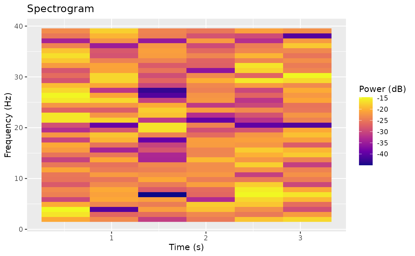
plotSpectrogram(spec, freq_range = c(1, 40))