Tutorial: Simulating Dynamic Synergy Data with Three Control Axes

Overview

The simulate_dynamic_synergy_data() function provides a powerful framework for generating synthetic muscle synergy data with controlled characteristics. Unlike traditional simulation approaches that generate data from a single global model, this function enables researchers to systematically explore how different motor control strategies affect muscle synergy structures through three orthogonal control axes.

Three Orthogonal Control Axes

The simulation framework is built around three complementary dimensions of motor control diversity:

1. Spatial Structure (cluster_sep_spatial): Controls how muscle groups contribute to synergy components. This axis defines the spatial organization of muscle activation patterns, such as proximal-dominant (hip and thigh emphasis), distal-dominant (calf and shin emphasis), or balanced patterns. In rehabilitation contexts, this might represent different movement strategies adopted by patients with varying levels of motor impairment.

2. Temporal Coordination (cluster_sep_temporal): Governs the timing and rhythmic properties of synergy activations. This includes onset timing, phase relationships, and frequency characteristics. Three representative coordination modes are implemented: - Rigid/Co-contraction: All synergies activate in-phase with strong temporal overlap - Alternating/Efficient: Phases evenly distributed with minimal overlap - Adaptive/Reactive: Random phases with heterogeneous frequencies

3. Stability-Adaptability (cluster_sep_stability): Introduces physiological and measurement variability to simulate differences in motor control precision. This axis represents the trade-off between stable, precise control (characteristic of elite athletes or late-stage rehabilitation) and adaptive, exploratory control (characteristic of early rehabilitation or fatigue states).

Each axis can be independently controlled with separation parameters ranging from 0 (no differentiation between clusters) to 2 (strongly distinct patterns), enabling factorial experimental designs.

Simulation Setup

Let’s begin by loading the required packages and generating a basic dataset:

library(synergyMixR)
library(ggplot2)
library(patchwork)
if (requireNamespace("viridis", quietly = TRUE)) {
  library(viridis)  # Required for plot_synergy_bases color scales
}

set.seed(650)
sim <- simulate_dynamic_synergy_data(
  N = 30,           # 30 subjects
  K = 3,            # 3 clusters (subgroups)
  r = 3,            # 3 synergies per cluster
  M = 8,            # 8 muscles
  T_each = 200,     # 200 time points per subject
  cluster_sep_spatial = 1.0,
  cluster_sep_temporal = 1.0,
  cluster_sep_stability = 1.0
)

Let’s examine the structure of the returned object:

str(sim, max.level = 2)
#> List of 7
#>  $ X_list          :List of 30
#>   ..$ : num [1:200, 1:8] 0.305 0.584 0.105 0.297 0.759 ...
#>   ..$ : num [1:200, 1:8] 0.0307 0.748 0.2039 0.258 0.1611 ...
#>   ..$ : num [1:200, 1:8] 0.0826 0.3029 0.3112 0.182 0.207 ...
#>   ..$ : num [1:200, 1:8] 0 0.1208 0.1082 0.0237 0.0634 ...
#>   ..$ : num [1:200, 1:8] 0.2013 0.4149 0.3264 0.0379 0.1517 ...
#>   ..$ : num [1:200, 1:8] 0 0 0.00332 0 0 ...
#>   ..$ : num [1:200, 1:8] 0.03337 0.04751 0.07669 0 0.00873 ...
#>   ..$ : num [1:200, 1:8] 0 0.00386 0.02293 0.08338 0 ...
#>   ..$ : num [1:200, 1:8] 0.297 0.321 0.143 0.289 0.059 ...
#>   ..$ : num [1:200, 1:8] 0.0193 0.0361 0.039 0.0664 0.0977 ...
#>   ..$ : num [1:200, 1:8] 0.07603 0.01616 0.00142 0.07762 0 ...
#>   ..$ : num [1:200, 1:8] 0.0292 0.0698 0.0905 0.1667 0.051 ...
#>   ..$ : num [1:200, 1:8] 0.0129 0.0553 0.1085 0.0939 0 ...
#>   ..$ : num [1:200, 1:8] 0.3038 0.056 0.2256 0.169 0.0759 ...
#>   ..$ : num [1:200, 1:8] 0.29565 0.31574 0.2375 0.41094 0.00827 ...
#>   ..$ : num [1:200, 1:8] 0.0515 0.0547 0.0882 0.0414 0.0179 ...
#>   ..$ : num [1:200, 1:8] 0 0.238 0.107 0.043 0.21 ...
#>   ..$ : num [1:200, 1:8] 0.218 0.324 0.292 0.12 0.326 ...
#>   ..$ : num [1:200, 1:8] 0.0884 0.1353 0.0468 0.0921 0.0946 ...
#>   ..$ : num [1:200, 1:8] 0.0188 0.1653 0.0851 0.1227 0.0866 ...
#>   ..$ : num [1:200, 1:8] 0 0.0297 0.027 0.0426 0.1447 ...
#>   ..$ : num [1:200, 1:8] 0.000761 0.033978 0.045855 0.049381 0.143597 ...
#>   ..$ : num [1:200, 1:8] 0.11 0.266 0.218 0.285 0.26 ...
#>   ..$ : num [1:200, 1:8] 0.11576 0.13539 0.15333 0.00643 0.02861 ...
#>   ..$ : num [1:200, 1:8] 0.176 0.281 0 0.317 0.213 ...
#>   ..$ : num [1:200, 1:8] 0.08346 0 0.13122 0.00815 0.08794 ...
#>   ..$ : num [1:200, 1:8] 0.0453 0.0581 0.0162 0.0443 0.0554 ...
#>   ..$ : num [1:200, 1:8] 0.3024 0.0321 0.168 0.1331 0.127 ...
#>   ..$ : num [1:200, 1:8] 0.365 0.35 0.227 0.261 0 ...
#>   ..$ : num [1:200, 1:8] 0.1826 0.0986 0 0.0571 0 ...
#>  $ C_list          :List of 30
#>   ..$ : num [1:200, 1:3] 0.57 0.383 0.651 0.581 0.615 ...
#>   ..$ : num [1:200, 1:3] 0.568 0.701 0.844 0.827 0.893 ...
#>   ..$ : num [1:200, 1:3] 0.626 0.505 0.583 0.822 0.664 ...
#>   ..$ : num [1:200, 1:3] 0.709 0.604 0.618 0.251 0.199 ...
#>   ..$ : num [1:200, 1:3] 0.637 0.94 0.761 1.106 0.946 ...
#>   ..$ : num [1:200, 1:3] 0.4566 0.2844 0.2998 0.0959 0.1191 ...
#>   ..$ : num [1:200, 1:3] 0.502 0.594 0.231 0.297 0.344 ...
#>   ..$ : num [1:200, 1:3] 0.559 0.158 0.394 0.152 0.142 ...
#>   ..$ : num [1:200, 1:3] 0.443 0.435 0.437 0.467 0.52 ...
#>   ..$ : num [1:200, 1:3] 0.05 0.1441 0.2995 0.1343 0.0908 ...
#>   ..$ : num [1:200, 1:3] 0.563 0.527 0.561 0.447 0.245 ...
#>   ..$ : num [1:200, 1:3] 0.289 0.301 0.234 0.129 0.156 ...
#>   ..$ : num [1:200, 1:3] 0.151 0.139 0.208 0.137 0.088 ...
#>   ..$ : num [1:200, 1:3] 0.57 0.344 0.421 0.322 0.231 ...
#>   ..$ : num [1:200, 1:3] 0.852 0.631 1.055 1.078 0.858 ...
#>   ..$ : num [1:200, 1:3] 0.05 0.208 0.14 0.05 0.132 ...
#>   ..$ : num [1:200, 1:3] 0.602 0.651 0.645 0.726 0.594 ...
#>   ..$ : num [1:200, 1:3] 0.591 0.625 0.634 0.76 0.745 ...
#>   ..$ : num [1:200, 1:3] 0.1417 0.1864 0.2409 0.0794 0.1596 ...
#>   ..$ : num [1:200, 1:3] 0.05 0.525 0.123 0.281 0.268 ...
#>   ..$ : num [1:200, 1:3] 0.05 0.1757 0.05 0.0518 0.1784 ...
#>   ..$ : num [1:200, 1:3] 0.05 0.1274 0.0683 0.08 0.1969 ...
#>   ..$ : num [1:200, 1:3] 0.564 0.36 0.49 0.656 0.485 ...
#>   ..$ : num [1:200, 1:3] 0.663 0.688 0.298 0.397 0.206 ...
#>   ..$ : num [1:200, 1:3] 0.546 1.114 0.819 0.752 1.013 ...
#>   ..$ : num [1:200, 1:3] 0.441 0.252 0.369 0.209 0.238 ...
#>   ..$ : num [1:200, 1:3] 0.105 0.146 0.175 0.206 0.121 ...
#>   ..$ : num [1:200, 1:3] 0.453 0.635 0.452 0.307 0.377 ...
#>   ..$ : num [1:200, 1:3] 0.457 0.607 0.615 0.72 0.745 ...
#>   ..$ : num [1:200, 1:3] 0.909 0.919 0.612 0.405 0.521 ...
#>  $ Lambda_list     :List of 3
#>   ..$ : num [1:8, 1:3] 0.239 0.2427 0.2021 0.0735 0.0922 ...
#>   ..$ : num [1:8, 1:3] 0.105 0.0992 0.0525 0.1251 0.0386 ...
#>   ..$ : num [1:8, 1:3] 0.1569 0.2343 0.1414 0.1469 0.0387 ...
#>  $ z_true          : int [1:30] 3 3 3 2 3 2 2 2 3 1 ...
#>  $ spatial_params  :List of 3
#>   ..$ :List of 1
#>   ..$ :List of 1
#>   ..$ :List of 1
#>  $ temporal_params :List of 3
#>   ..$ :List of 5
#>   ..$ :List of 5
#>   ..$ :List of 5
#>  $ stability_params:List of 3
#>   ..$ :List of 4
#>   ..$ :List of 4
#>   ..$ :List of 4

The simulation returns a list containing:

X_list: EMG signals for each subject (T × M matrices)
C_list: Synergy activation signals for each subject (T × r matrices)
Lambda_list: Cluster-specific synergy loading matrices (M × r matrices)
z_true: True cluster assignments for each subject
spatial_params: Spatial structure parameters for each cluster
temporal_params: Temporal coordination parameters for each cluster
stability_params: Stability-adaptability parameters for each cluster

cat("Cluster distribution:\n")
#> Cluster distribution:
table(sim$z_true)
#> 
#>  1  2  3 
#>  8 11 11

Visualization

The package provides six visualization functions to explore different aspects of the simulated data.

Synergy Bases (Spatial Structure)

The plot_synergy_bases() function visualizes the synergy loading matrices (Lambda_k) for each cluster as heatmaps. Each heatmap shows how strongly each muscle contributes to each synergy component.

plot_synergy_bases(sim)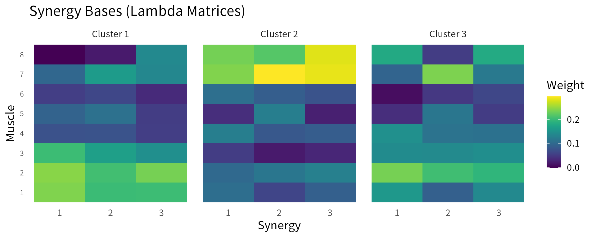

Interpretation: The heatmaps reveal the spatial organization of muscle synergies. Cluster 1 shows proximal-dominant patterns (stronger weights in the first few muscles), Cluster 2 shows distal-dominant patterns (stronger weights in the last few muscles), and Cluster 3 shows a more balanced or mixed pattern. These differences reflect distinct motor control strategies that might be observed in different patient populations or skill levels.

Temporal Activation Patterns

The plot_activation_patterns() function shows how synergies are activated over time for representative subjects from each cluster.

plot_activation_patterns(sim)

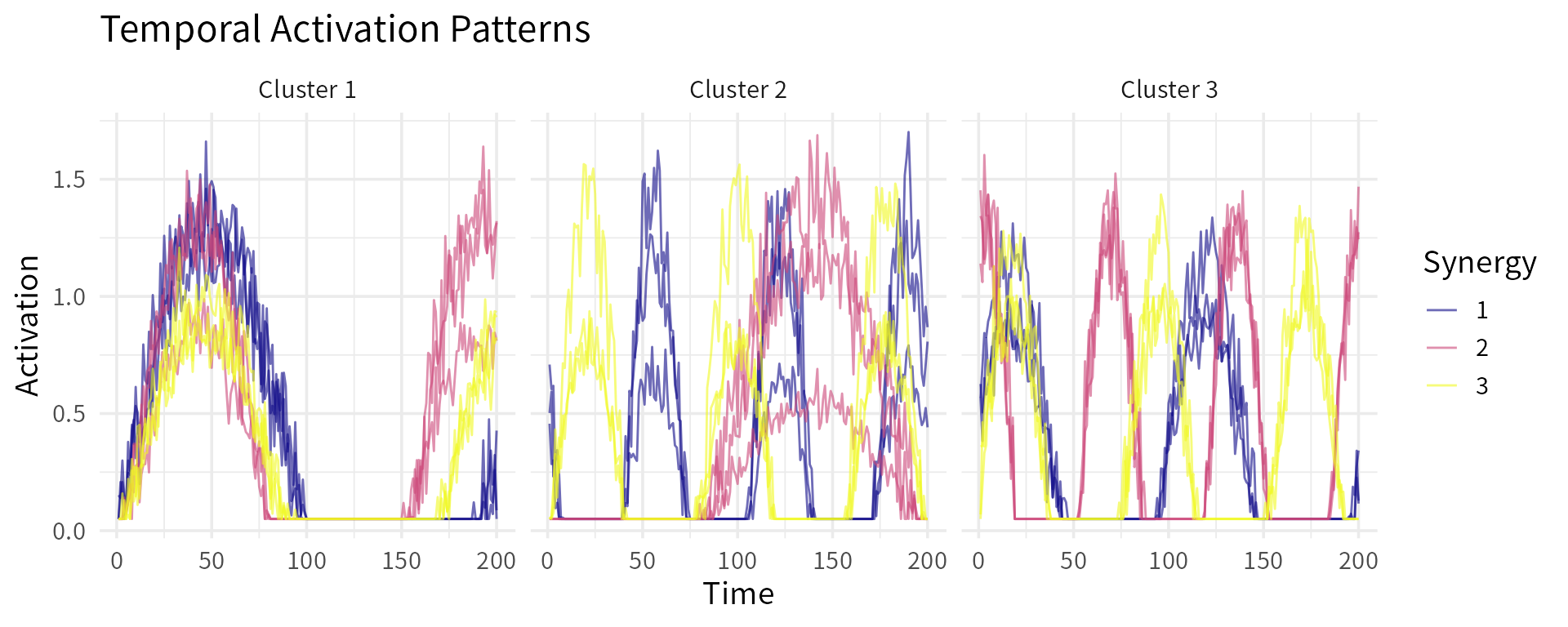
Interpretation: The temporal patterns reveal coordination differences between clusters. Notice how the timing, phase relationships, and rhythmic properties differ across clusters. Cluster 1 may show more synchronized activation (co-contraction), Cluster 2 may show alternating patterns (efficient coordination), and Cluster 3 may show more variable timing (adaptive control).

Reconstructed EMG Signals

The plot_reconstructed_emg() function displays the full EMG time-series for all subjects and muscles. Individual subject traces appear as thin semi-transparent lines, while the cluster-mean waveform is shown as a bold black line.

plot_reconstructed_emg(sim)

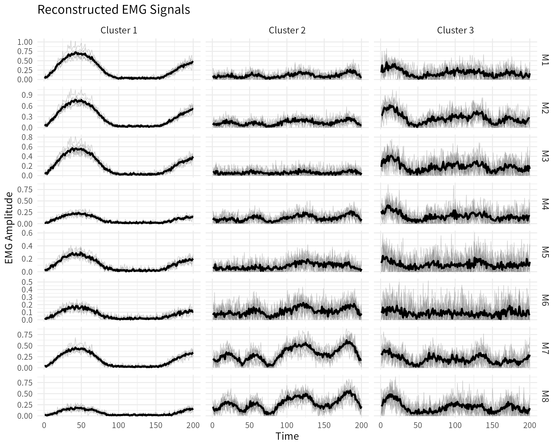
Interpretation: This visualization reveals both the underlying synergy structure (reflected in the mean waveforms) and the inter-subject variability within each cluster. The spread of individual traces around the mean indicates the degree of motor variability, which may reflect differences in motor learning stage, fatigue, or control strategy.

Noise Profiles (Stability-Adaptability)

The plot_noise_profiles() function shows the distribution of noise parameters across clusters, revealing differences in control precision and adaptability.

plot_noise_profiles(sim)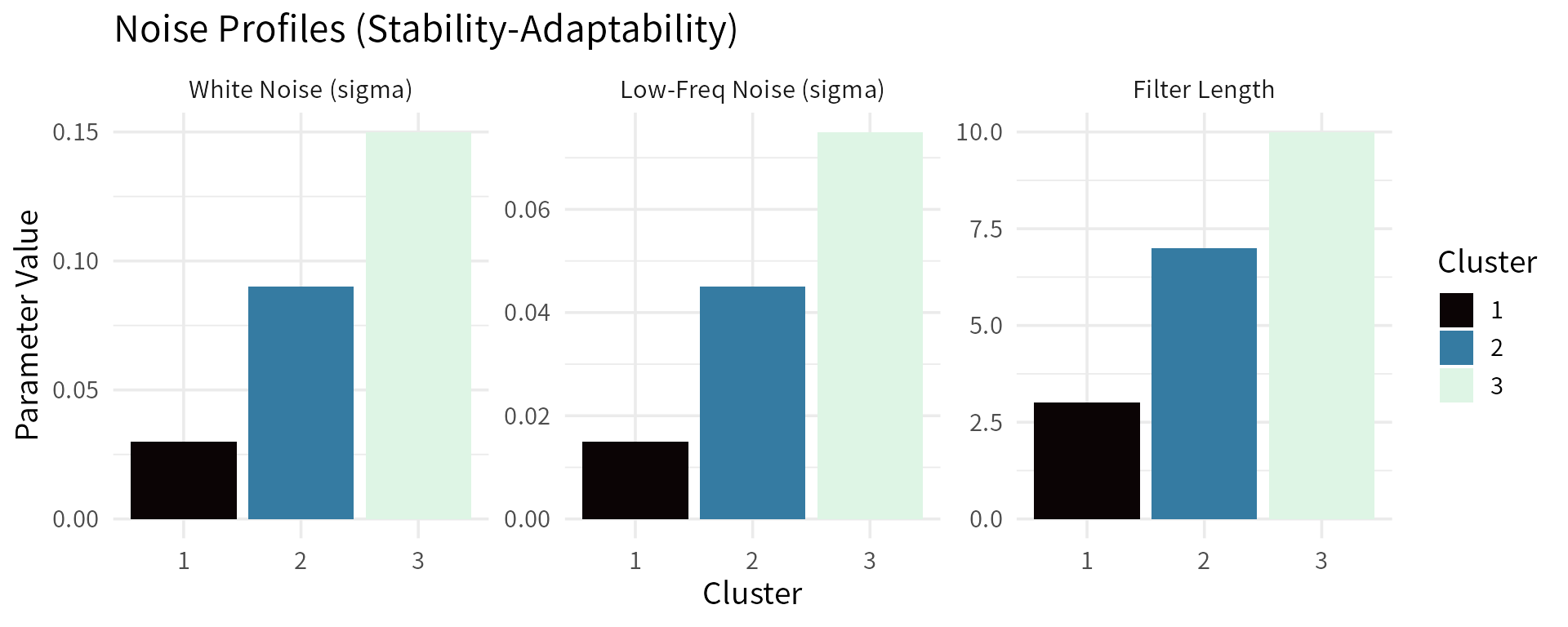

Interpretation: The noise profiles quantify the stability-adaptability trade-off. Cluster 1 (stable control) shows low noise levels, indicating precise, consistent motor control. Cluster 3 (adaptive control) shows higher noise levels, indicating more variable, exploratory control. These differences might correspond to different stages of motor learning or rehabilitation.

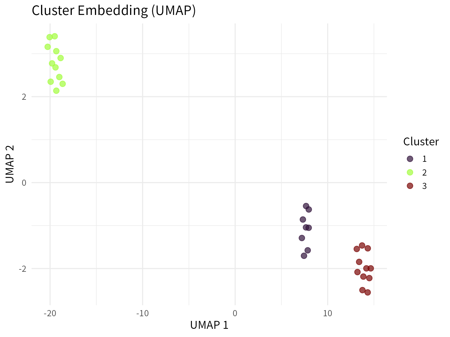
Cluster Embedding (Separability)

The plot_cluster_embedding() function creates a low-dimensional visualization of cluster separability using UMAP or PCA. Each point represents a subject, colored by true cluster assignment.

# UMAP embedding (if umap package is available)
if (requireNamespace("umap", quietly = TRUE)) {
  plot_cluster_embedding(sim, method = "umap")
}

# PCA embedding (always available)
plot_cluster_embedding(sim, method = "pca")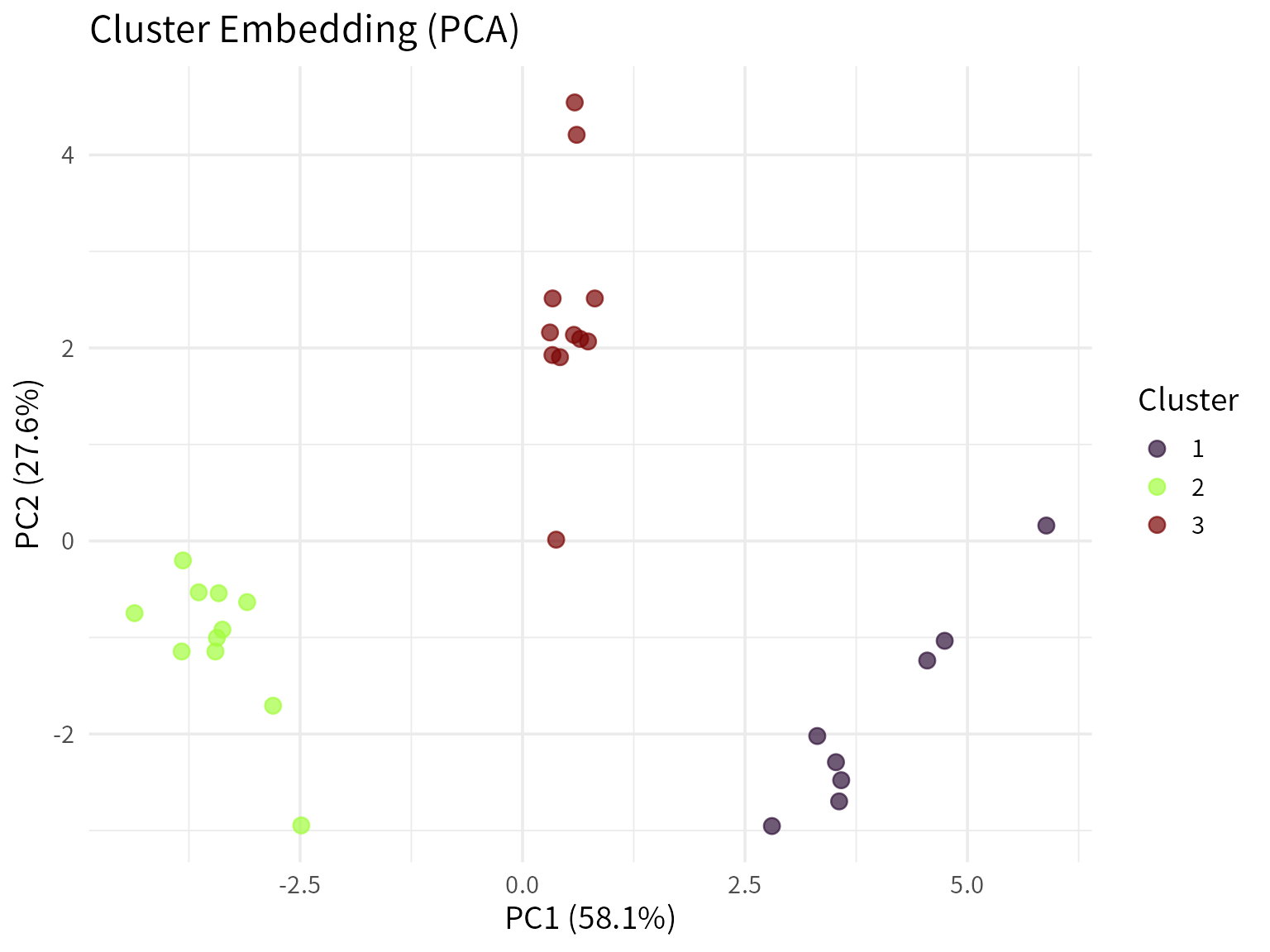

Interpretation: The embedding reveals how well-separated the clusters are in feature space. Well-separated clusters indicate that the three control axes have created distinct motor control profiles. This visualization is useful for assessing whether the simulated data will be challenging or easy for clustering algorithms to recover.

Comprehensive Summary

The plot_synergy_summary() function combines multiple visualization panels into a single comprehensive overview using the patchwork package.

if (requireNamespace("patchwork", quietly = TRUE)) {
  plot_synergy_summary(sim)
}

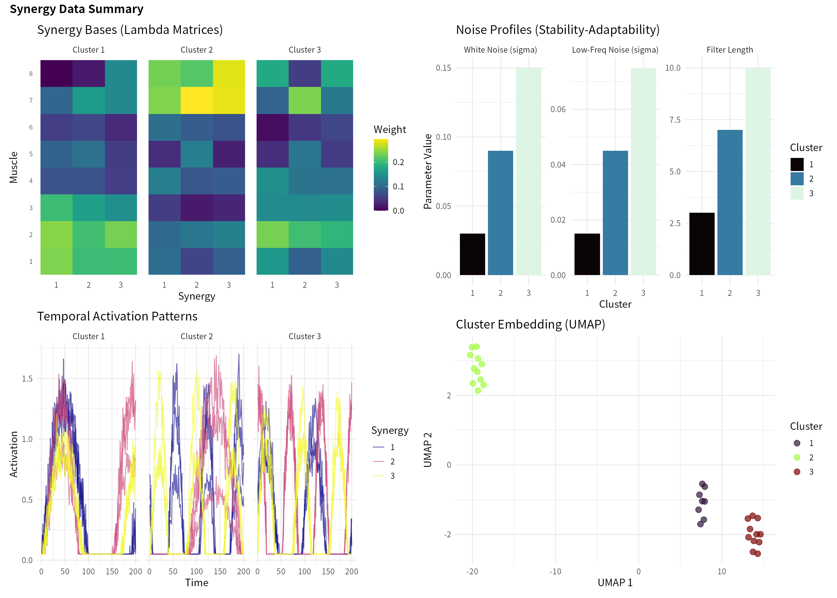
Interpretation: This summary provides a holistic view of the simulated data, showing spatial synergy structures (top left), temporal activation dynamics (top right), noise profiles (bottom left), and cluster separability (bottom right). This is particularly useful for quickly assessing the overall characteristics of a simulation.

Neural Command Visualization

The plot_neural_command() function visualizes the temporal evolution of neural control signals by creating a low-dimensional representation of synergy activation trajectories. This reveals how motor commands change over time within and across clusters.

plot_neural_command(sim, method = "pca", color_by = "cluster", smooth = TRUE)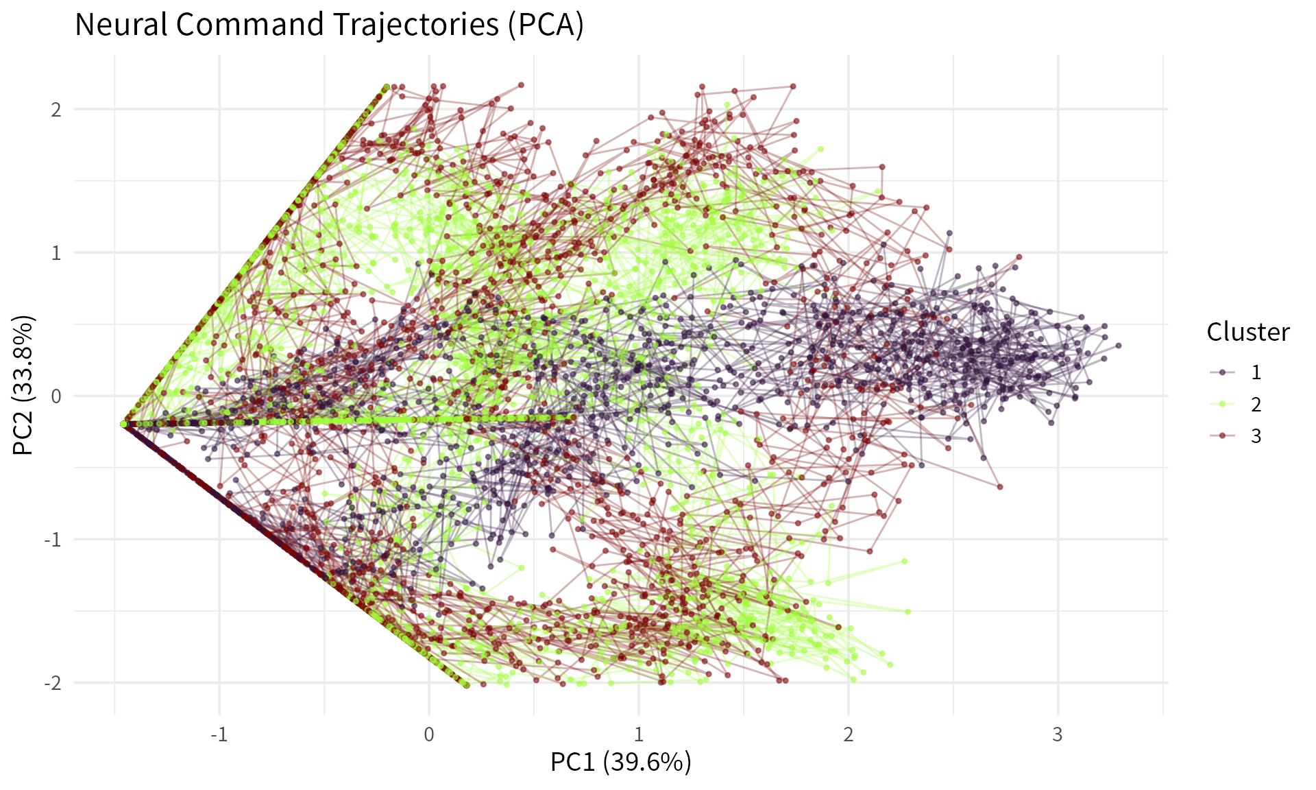

Interpretation: The neural command embedding reveals temporal evolution of control signals across clusters, showing coherent trajectories for shared synergy activation patterns. Each trajectory represents how a subject’s neural commands evolve through time, with smooth paths connecting consecutive time points. Clusters with distinct temporal coordination strategies (co-contraction vs. alternating vs. adaptive) form separate regions in this low-dimensional space.

We can also visualize the temporal progression by coloring points by time rather than cluster:

plot_neural_command(sim, method = "pca", color_by = "time", smooth = TRUE)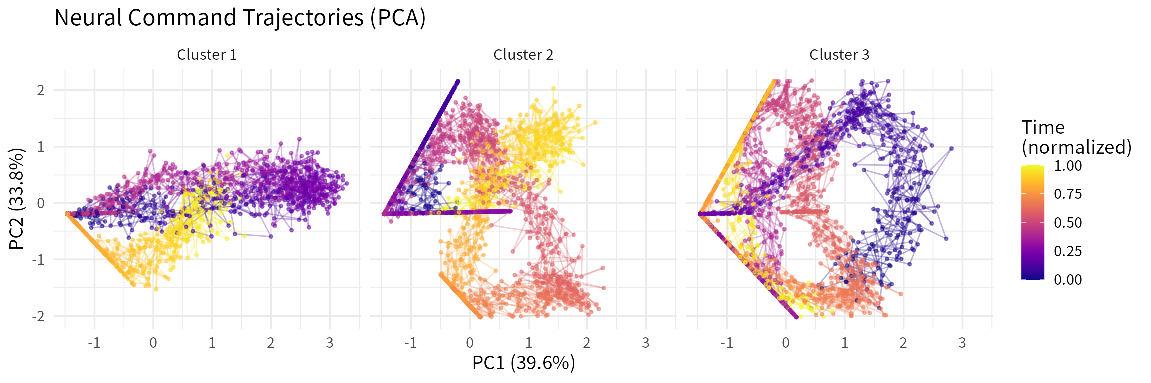

Interpretation: When colored by time, the trajectories reveal how neural commands evolve from the beginning (dark purple) to the end (bright yellow) of each movement cycle. This visualization is particularly useful for identifying periodic patterns, transient dynamics, or drift in motor control strategies over time. The faceting by cluster allows direct comparison of temporal evolution patterns across different motor control strategies.

If the uwot package is available, we can also use UMAP for a potentially more informative embedding:

if (requireNamespace("uwot", quietly = TRUE)) {
  plot_neural_command(sim, method = "umap", color_by = "cluster", smooth = TRUE)
}

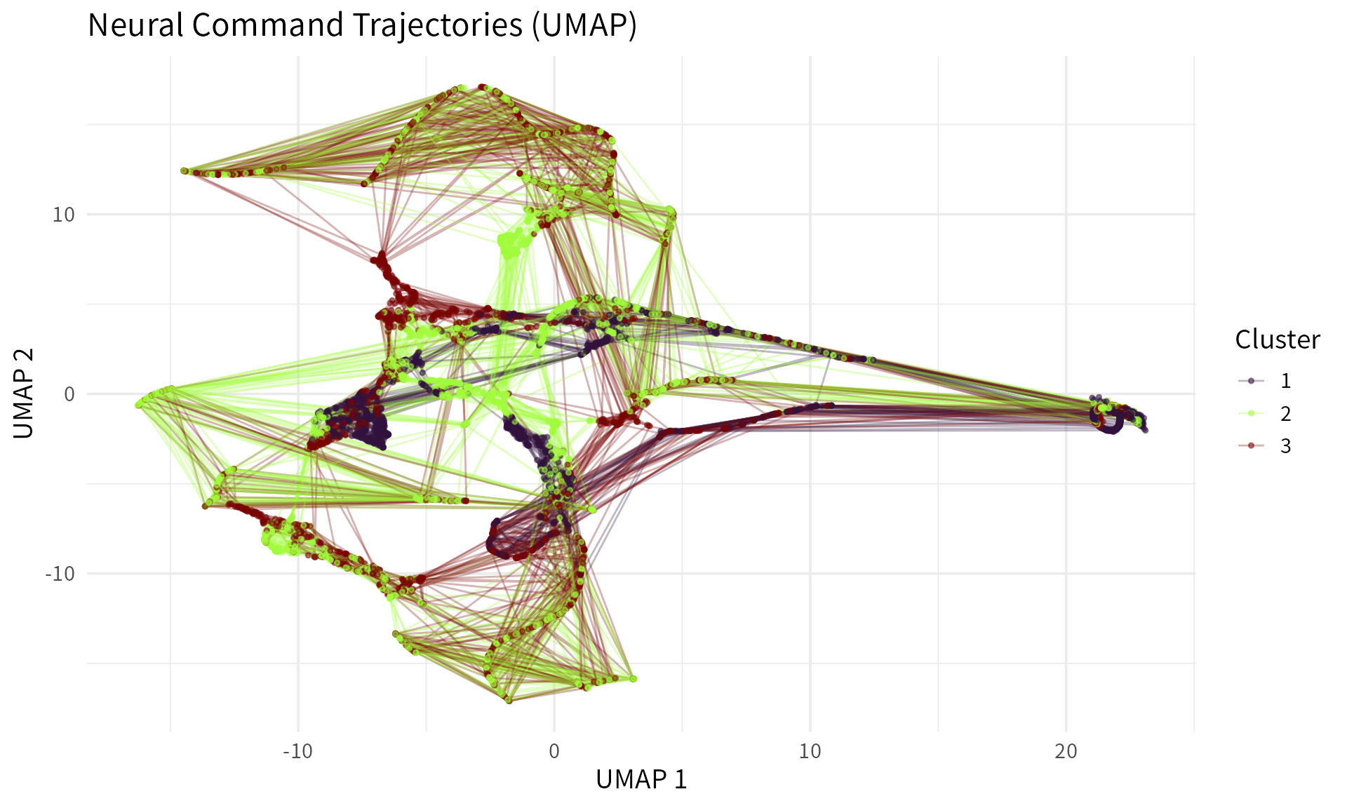
Interpretation: UMAP often provides better separation of clusters and can reveal nonlinear structure in the neural command space that PCA might miss. The smooth trajectories show how individual subjects navigate through the neural command space over time, with cluster-specific patterns emerging as distinct regions or pathways.

Cluster-Wise Subject Distribution

To examine the distribution of subjects within a specific cluster, we can use the cluster_id parameter:

plot_reconstructed_emg(sim, cluster_id = 1)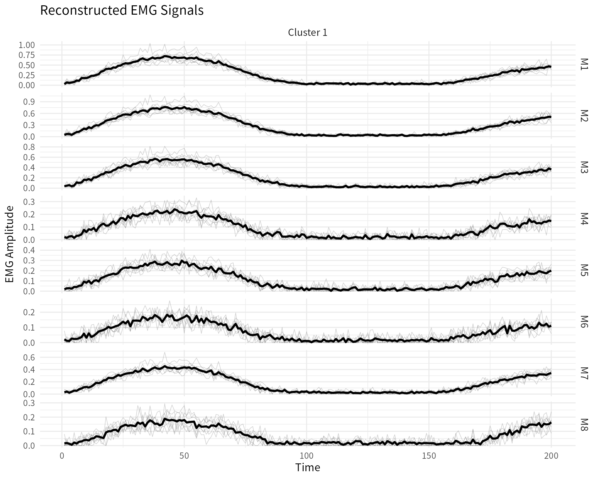

Interpretation: This view shows all subjects from Cluster 1 (faint gray lines) overlaid with the cluster mean (bold black line). The variability around the mean reflects individual differences in motor execution while maintaining the same underlying synergy structure. This type of visualization is valuable for understanding how much within-cluster variability exists and whether the cluster represents a coherent motor strategy.

Let’s examine another cluster:

plot_reconstructed_emg(sim, cluster_id = 2)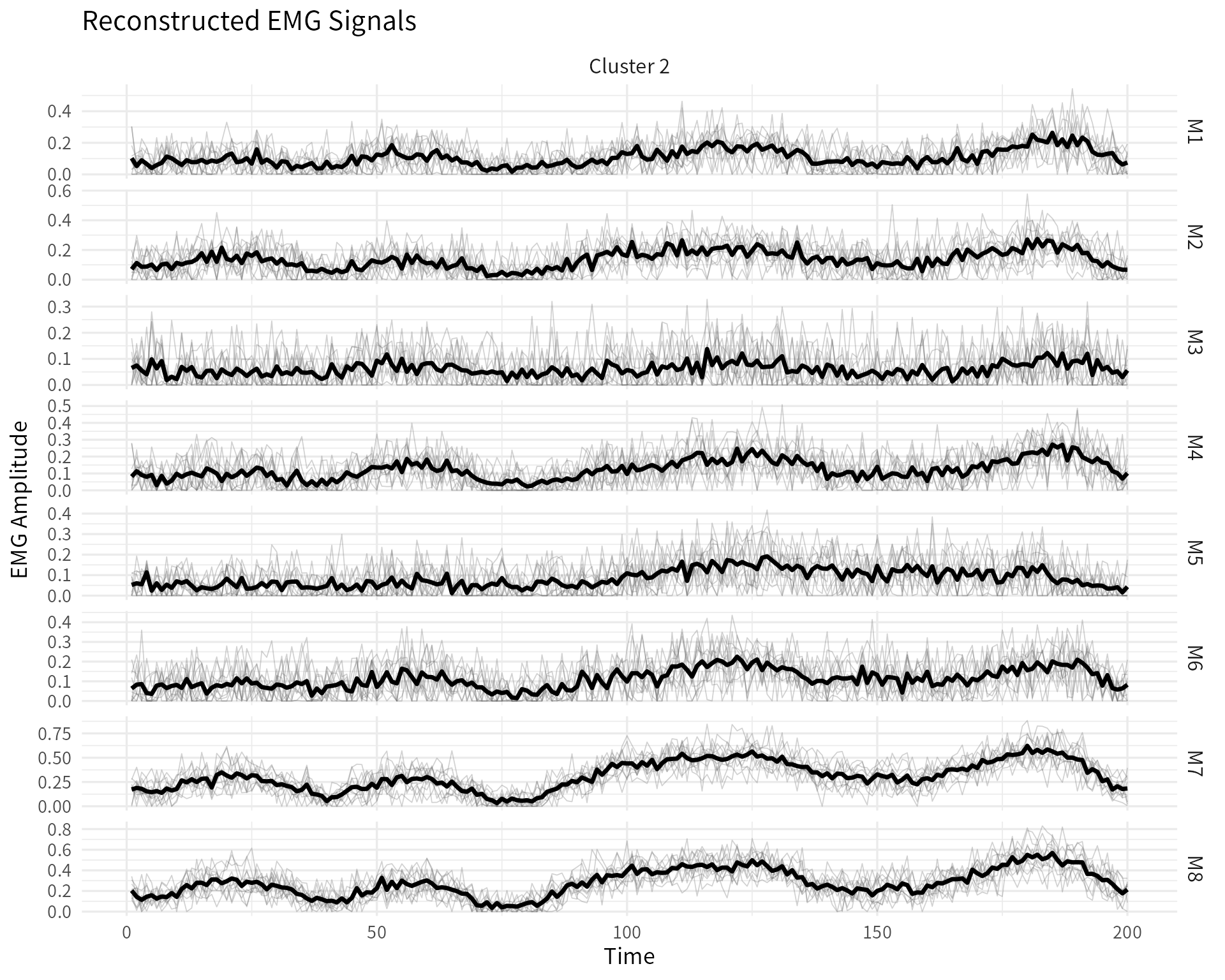

We can also focus on specific muscles:

plot_reconstructed_emg(sim, cluster_id = 1, muscles = c(1, 2, 3, 4))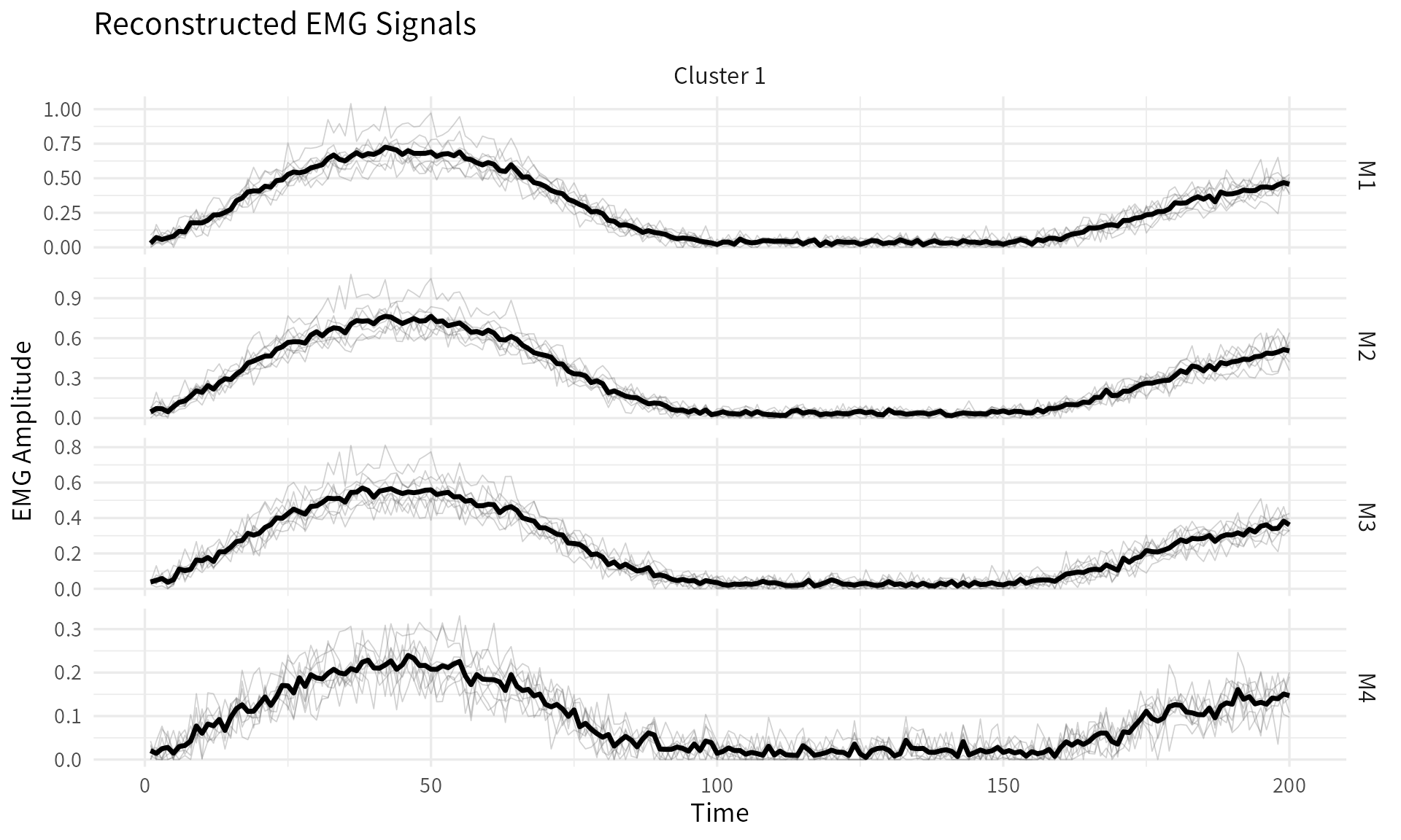

Interpretation: By focusing on a subset of muscles, we can more clearly see the temporal patterns and inter-subject variability in specific muscle groups. This is useful when investigating hypotheses about specific muscle coordination patterns.

Exploring Control-Axis Effects

One of the key advantages of simulate_dynamic_synergy_data() is the ability to systematically explore how each control axis affects the data characteristics. Let’s sweep one axis at a time while holding the others constant.

Effect of Spatial Separation

spatial_levels <- c(0, 0.5, 1.0, 2.0)
sims_spatial <- lapply(spatial_levels, function(sep) {
  simulate_dynamic_synergy_data(
    N = 20, K = 3, r = 3, M = 8, T_each = 100,
    cluster_sep_spatial = sep,
    cluster_sep_temporal = 1.0,
    cluster_sep_stability = 1.0,
    seed = 700
  )
})

# Visualize synergy bases across spatial separation levels
plots_spatial <- lapply(seq_along(spatial_levels), function(i) {
  plot_synergy_bases(sims_spatial[[i]], theme_base_size = 10) +
    ggtitle(paste0("Spatial Sep = ", spatial_levels[i]))
})

if (requireNamespace("patchwork", quietly = TRUE)) {
  patchwork::wrap_plots(plots_spatial, nrow = 1)
}

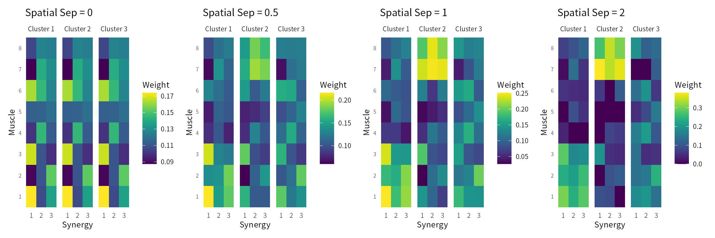
Interpretation: As spatial separation increases from 0 to 2, the synergy loading matrices become increasingly distinct across clusters. At separation = 0, all clusters have nearly identical spatial patterns. At separation = 2, the clusters show strongly differentiated muscle activation profiles.

Effect of Temporal Separation

temporal_levels <- c(0, 0.5, 1.0, 2.0)
sims_temporal <- lapply(temporal_levels, function(sep) {
  simulate_dynamic_synergy_data(
    N = 20, K = 3, r = 3, M = 8, T_each = 100,
    cluster_sep_spatial = 1.0,
    cluster_sep_temporal = sep,
    cluster_sep_stability = 1.0,
    seed = 800
  )
})

# Visualize activation patterns across temporal separation levels
plots_temporal <- lapply(seq_along(temporal_levels), function(i) {
  plot_activation_patterns(sims_temporal[[i]], theme_base_size = 10) +
    ggtitle(paste0("Temporal Sep = ", temporal_levels[i]))
})

if (requireNamespace("patchwork", quietly = TRUE)) {
  patchwork::wrap_plots(plots_temporal, nrow = 1)
}

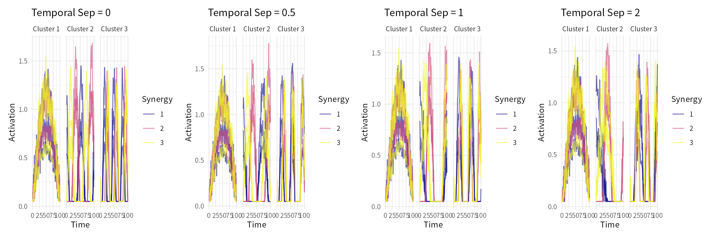
Interpretation: As temporal separation increases, the phase relationships and frequency characteristics become more distinct across clusters. At low separation, all clusters show similar temporal coordination. At high separation, the clusters exhibit clearly different timing patterns (co-contraction vs. alternating vs. adaptive).

Effect of Stability Separation

stability_levels <- c(0, 0.5, 1.0, 2.0)
sims_stability <- lapply(stability_levels, function(sep) {
  simulate_dynamic_synergy_data(
    N = 20, K = 3, r = 3, M = 8, T_each = 100,
    cluster_sep_spatial = 1.0,
    cluster_sep_temporal = 1.0,
    cluster_sep_stability = sep,
    seed = 900
  )
})

# Visualize noise profiles across stability separation levels
plots_stability <- lapply(seq_along(stability_levels), function(i) {
  plot_noise_profiles(sims_stability[[i]], theme_base_size = 10) +
    ggtitle(paste0("Stability Sep = ", stability_levels[i]))
})

if (requireNamespace("patchwork", quietly = TRUE)) {
  patchwork::wrap_plots(plots_stability, nrow = 1)
}

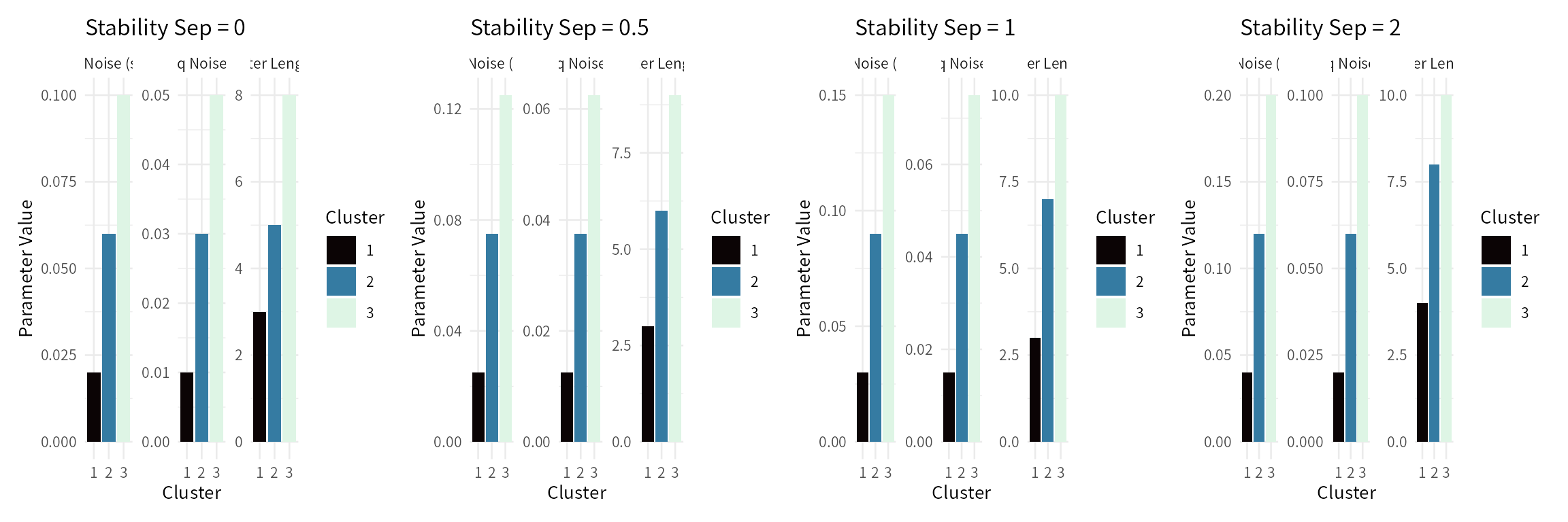
Interpretation: As stability separation increases, the noise characteristics become more differentiated across clusters. At low separation, all clusters have similar noise levels. At high separation, the clusters show clearly distinct stability profiles, ranging from precise control to adaptive/exploratory control.

Combined Effect on Cluster Separability

Let’s examine how varying all three axes simultaneously affects cluster separability:

# Create a grid of parameter combinations
param_grid <- expand.grid(
  spatial = c(0.5, 1.5),
  temporal = c(0.5, 1.5),
  stability = c(0.5, 1.5)
)

sims_combined <- lapply(seq_len(nrow(param_grid)), function(i) {
  simulate_dynamic_synergy_data(
    N = 20, K = 3, r = 3, M = 8, T_each = 100,
    cluster_sep_spatial = param_grid$spatial[i],
    cluster_sep_temporal = param_grid$temporal[i],
    cluster_sep_stability = param_grid$stability[i],
    seed = 1000 + i
  )
})

# Visualize embeddings
plots_combined <- lapply(seq_len(nrow(param_grid)), function(i) {
  title <- sprintf("Sp=%.1f, Tp=%.1f, St=%.1f",
                   param_grid$spatial[i],
                   param_grid$temporal[i],
                   param_grid$stability[i])
  plot_cluster_embedding(sims_combined[[i]], method = "pca", theme_base_size = 9) +
    ggtitle(title)
})

if (requireNamespace("patchwork", quietly = TRUE)) {
  patchwork::wrap_plots(plots_combined, nrow = 2)
}

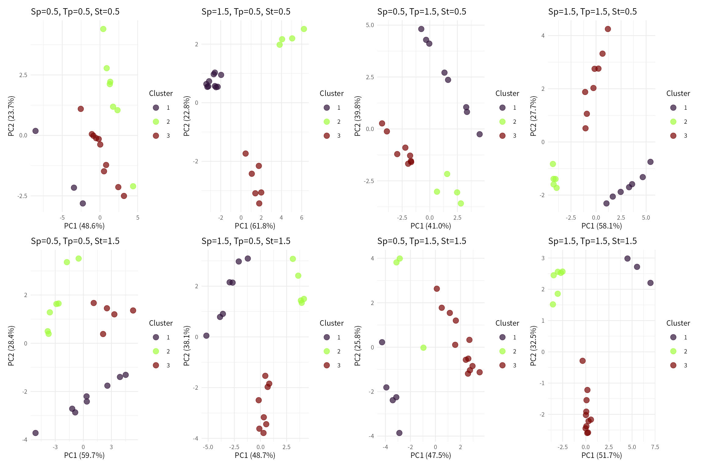
Interpretation: This factorial design reveals how the three control axes interact to determine overall cluster separability. When all three axes have high separation values, clusters are maximally distinct. When all have low values, clusters overlap considerably. Intermediate combinations produce varying degrees of separability, which can be used to create simulation scenarios of different difficulty levels for testing clustering algorithms.

Interpretation

The three control axes provide a principled framework for understanding and simulating motor control diversity:

Spatial Axis: Muscle Recruitment Strategies

The spatial axis captures differences in which muscle groups are preferentially recruited. In real-world contexts:

Proximal-dominant patterns might represent strategies that rely heavily on hip and trunk muscles, common in individuals with distal weakness or in power-focused movements
Distal-dominant patterns might represent strategies emphasizing ankle and foot control, common in precision tasks or in individuals with proximal weakness
Balanced patterns might represent well-coordinated strategies that distribute load across muscle groups

Temporal Axis: Coordination Strategies

The temporal axis captures differences in how muscles are coordinated over time:

Co-contraction (rigid) represents simultaneous activation of multiple muscle groups, providing stability but at the cost of efficiency. This is common in novice performers or in unstable conditions
Alternating (efficient) represents sequential activation with minimal overlap, maximizing efficiency. This is characteristic of skilled performers in rhythmic tasks
Adaptive (reactive) represents variable timing patterns that allow flexibility in response to changing task demands, common in complex or unpredictable environments

Stability Axis: Control Precision vs. Adaptability

The stability axis captures the trade-off between precise, consistent control and flexible, adaptive control:

Stable control (low noise) represents highly practiced, automated movements with minimal variability. This is characteristic of elite athletes or late-stage rehabilitation patients
Moderate control represents a balance between consistency and flexibility
Adaptive control (high noise) represents exploratory, variable movements that allow learning and adaptation. This is characteristic of early-stage learning or rehabilitation

Factorial Design Possibilities

By independently manipulating these three axes, researchers can create factorial designs to investigate:

Algorithm robustness: Test whether clustering algorithms can recover true structure under varying levels of separation
Feature importance: Determine which aspects of motor control (spatial, temporal, stability) are most informative for subgroup identification
Sample size requirements: Assess how many subjects are needed to reliably detect clusters with different separation characteristics
Model selection: Compare different mixture models (MFA, MPCA, etc.) under controlled conditions

Reproducibility

All simulations in this tutorial are fully reproducible through the use of random seeds. The simulation function and all visualization functions are thoroughly tested:

Simulation tests: tests/test_simulation_v2.R validates the three-axis control system
Visualization tests: tests/test_visualization_v2.R ensures all plotting functions generate proper outputs

These tests can be run using:

# Run simulation tests
source(system.file("tests", "test_simulation_v2.R", package = "synergyMixR"))

# Run visualization tests
source(system.file("tests", "test_visualization_v2.R", package = "synergyMixR"))

Integration with MFA/MPCA Analysis Pipelines

The simulated data can be directly used with the package’s mixture model fitting functions:

# Example: Fit MFA model to simulated data
mfa_fit <- mfa_em_fit(
  list_of_data = sim$X_list,
  K = 3,
  r = 3,
  n_init = 10,
  max_iter = 100
)

# Compare true vs. estimated cluster assignments
library(mclust)
ari <- adjustedRandIndex(sim$z_true, mfa_fit$z)
cat("Adjusted Rand Index:", ari, "\n")

# Visualize results with estimated clusters
plot_cluster_embedding(sim, fit = mfa_fit, method = "umap")

This integration enables comprehensive benchmarking studies where ground truth is known, allowing rigorous evaluation of model performance under controlled conditions.

Summary

The simulate_dynamic_synergy_data() function and accompanying visualization suite provide a powerful framework for:

Generating realistic synthetic data with controlled characteristics across three orthogonal dimensions of motor control
Visualizing complex patterns in spatial synergy structure, temporal coordination, and stability profiles
Conducting systematic studies through factorial designs that independently manipulate control axes
Benchmarking algorithms under known ground truth conditions
Exploring motor control theory by simulating different coordination strategies and control profiles

By providing fine-grained control over data characteristics while maintaining biological plausibility, this framework enables rigorous, reproducible research in muscle synergy analysis and motor control.

Session Information

sessionInfo()
#> R version 4.5.2 (2025-10-31)
#> Platform: x86_64-pc-linux-gnu
#> Running under: Ubuntu 24.04.4 LTS
#> 
#> Matrix products: default
#> BLAS:   /opt/R/4.5.2/lib/R/lib/libRblas.so 
#> LAPACK: /opt/R/4.5.2/lib/R/lib/libRlapack.so;  LAPACK version 3.12.1
#> 
#> locale:
#>  [1] LC_CTYPE=ja_JP.UTF-8       LC_NUMERIC=C              
#>  [3] LC_TIME=ja_JP.UTF-8        LC_COLLATE=ja_JP.UTF-8    
#>  [5] LC_MONETARY=ja_JP.UTF-8    LC_MESSAGES=ja_JP.UTF-8   
#>  [7] LC_PAPER=ja_JP.UTF-8       LC_NAME=C                 
#>  [9] LC_ADDRESS=C               LC_TELEPHONE=C            
#> [11] LC_MEASUREMENT=ja_JP.UTF-8 LC_IDENTIFICATION=C       
#> 
#> time zone: Asia/Tokyo
#> tzcode source: system (glibc)
#> 
#> attached base packages:
#> [1] stats     graphics  grDevices utils     datasets  methods   base     
#> 
#> other attached packages:
#> [1] viridis_0.6.5     viridisLite_0.4.3 patchwork_1.3.2   ggplot2_4.0.2    
#> [5] synergyMixR_1.0.0
#> 
#> loaded via a namespace (and not attached):
#>  [1] sass_0.4.10        generics_0.1.4     tidyr_1.3.2        lattice_0.22-7    
#>  [5] digest_0.6.39      magrittr_2.0.4     evaluate_1.0.5     grid_4.5.2        
#>  [9] RColorBrewer_1.1-3 fastmap_1.2.0      jsonlite_2.0.0     Matrix_1.7-4      
#> [13] umap_0.2.10.0      RSpectra_0.16-2    gridExtra_2.3      purrr_1.2.1       
#> [17] scales_1.4.0       codetools_0.2-20   textshaping_1.0.4  jquerylib_0.1.4   
#> [21] cli_3.6.5          rlang_1.1.7        RcppAnnoy_0.0.23   uwot_0.2.4        
#> [25] withr_3.0.2        cachem_1.1.0       yaml_2.3.12        FNN_1.1.4.1       
#> [29] otel_0.2.0         tools_4.5.2        dplyr_1.2.0        reticulate_1.45.0 
#> [33] png_0.1-8          vctrs_0.7.1        R6_2.6.1           lifecycle_1.0.5   
#> [37] fs_1.6.6           htmlwidgets_1.6.4  ragg_1.5.0         pkgconfig_2.0.3   
#> [41] desc_1.4.3         pkgdown_2.2.0      pillar_1.11.1      bslib_0.10.0      
#> [45] gtable_0.3.6       glue_1.8.0         Rcpp_1.1.1         systemfonts_1.3.1 
#> [49] xfun_0.56          tibble_3.3.1       tidyselect_1.2.1   knitr_1.51        
#> [53] farver_2.1.2       htmltools_0.5.9    rmarkdown_2.30     labeling_0.4.3    
#> [57] compiler_4.5.2     S7_0.2.1           askpass_1.2.1      openssl_2.3.4

synergyMixR Package

2026-08-14